
GA4 BigQuery Tutorial: How to Calculate 7-Day Moving Averages, Shares and DoD with SQL

I recently published a short video where I walk through a few SQL tricks in BigQuery that I use every day to get actionable insights from GA4 data. In this article I’ll expand on those ideas, explain the SQL patterns step-by-step, and show practical examples you can reuse. If you prefer a visual walkthrough, you can watch the full video tutorial embedded below or visit the YouTube channel:
Step 1: Prepare GA4 data in BigQuery (daily reports by day + source)
Before you do any of these calculations, you need a reliable daily table that aggregates GA4 events into one row per date and traffic source. I pull raw GA4 events into BigQuery, transform them with a scheduled query that runs every day, and save the results as a table called something like ga4_daily_reports_by_day_source.
The idea is to have at least these columns in the table:
- date — the day (DATE)
- source — traffic/source dimension (STRING)
- total_users — daily users per source (INTEGER)
- other metrics you want to analyze (sessions, revenue, purchases)
Having a daily aggregated table simplifies window functions and performance, because the SQL operates on rows per day rather than per event. You can use scheduled queries to keep this table up to date automatically. Once the table exists you’re ready to build moving averages, day shares and day-over-day deltas.
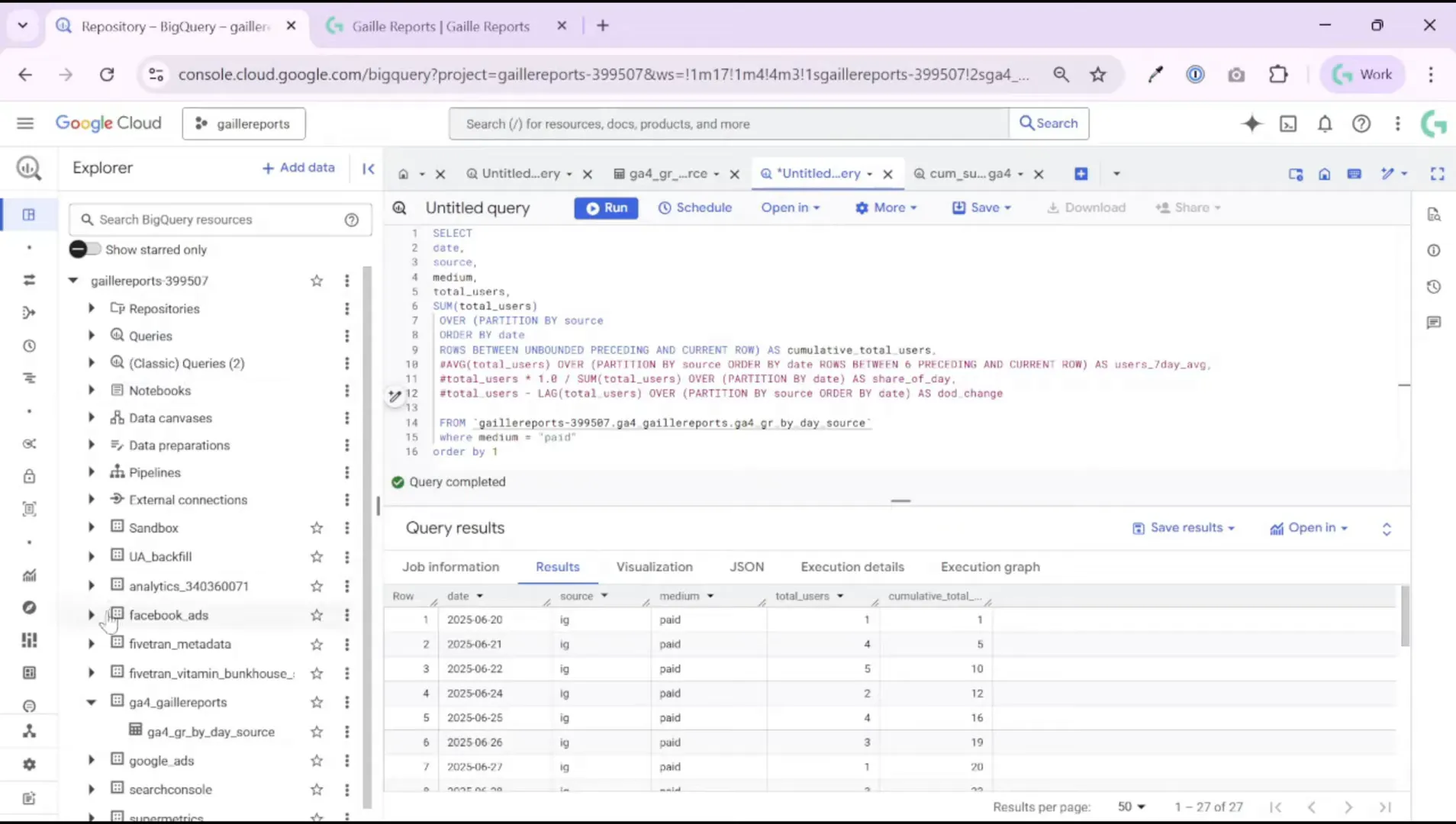
Step 2: Calculate a 7-day moving average per traffic source
One of the most useful metrics for marketing reporting is a rolling average. It smooths volatility and shows trends more clearly than raw daily numbers. In BigQuery, you can compute a 7-day moving average per source with a window function. The pattern looks like this in plain SQL terms:
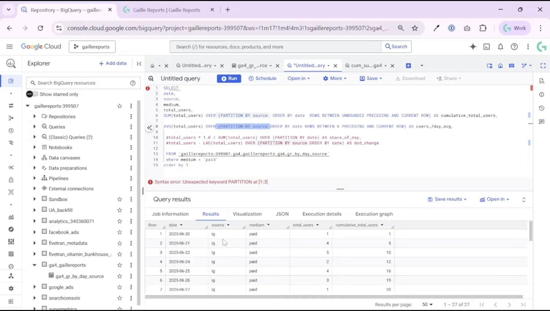
AVG(total_users) OVER (PARTITION BY source ORDER BY date ROWS BETWEEN 6 PRECEDING AND CURRENT ROW)Key points:
- PARTITION BY source makes the rolling average calculate separately for each traffic source (Instagram, Facebook, organic, etc.).
- ORDER BY date ensures the window respects chronological order.
- ROWS BETWEEN 6 PRECEDING AND CURRENT ROW defines a 7-day window (current day + 6 previous days).
Let me illustrate with numbers I used in my sample dataset. For one source (“instagram”) the daily total_users looked like this:
- 20 June — 1 user (average = 1 because only one day exists)
- 21 June — 4 users (cumulative total = 5 over 2 days, average = 2.5)
- 22 June — 5 users (cumulative total = 10 over 3 days, average ≈ 3.3)
As more days pass, the moving average becomes the average of the most recent seven days for that source. This smoothing is very useful when you have repeat purchasers or frequent returning users (e.g., food delivery apps, subscription products) because it highlights sustained changes rather than random spikes.
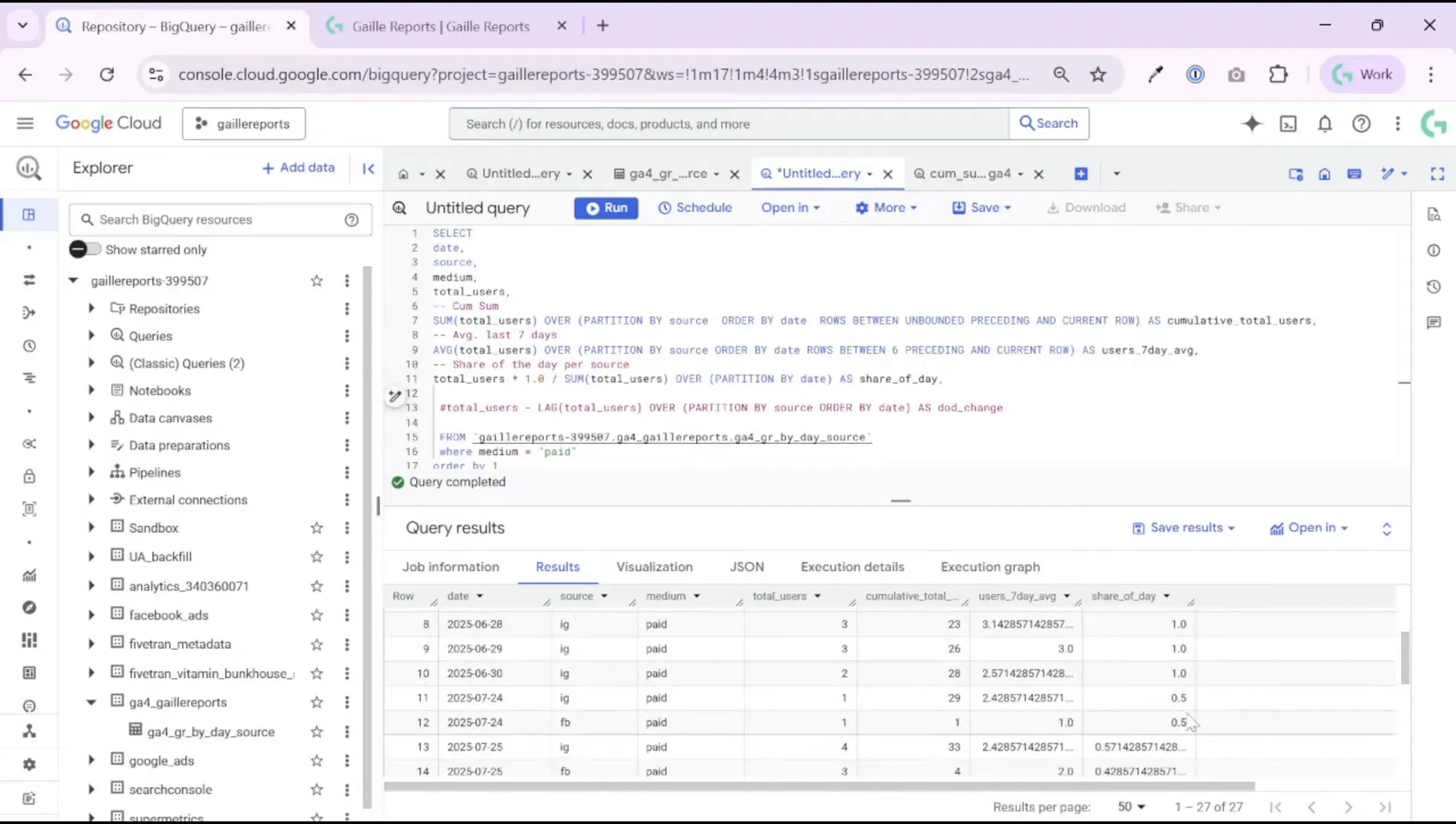
Step 3: Compute the daily share of each traffic source
To answer questions like “What share of today’s users came from Instagram?” use a simple ratio combined with a window sum across the same date. The pattern is:
(total_users * 1.0) / SUM(total_users) OVER (PARTITION BY date)Why multiply by 1.0? It coerces integers into floats so you get a decimal share (0.57 instead of integer division truncation). Using SUM(…) OVER (PARTITION BY date) returns the total users across all sources for that date, and dividing the source-specific total by that daily sum yields the share.
Example from the dataset:
- 24 July — 1 user from Instagram, 1 from Facebook → Instagram share = 1 / (1+1) = 50%.
- 25 July — 4 users from Instagram, 3 from Facebook → Instagram share = 4 / 7 ≈ 57%.
You can compute this share per day, per week, or for any other period by changing the partition and grouping logic. Use this metric to spot shifts in channel mix, e.g., whether paid campaigns are increasing their slice of daily users or whether organic regained share after a promotional push.
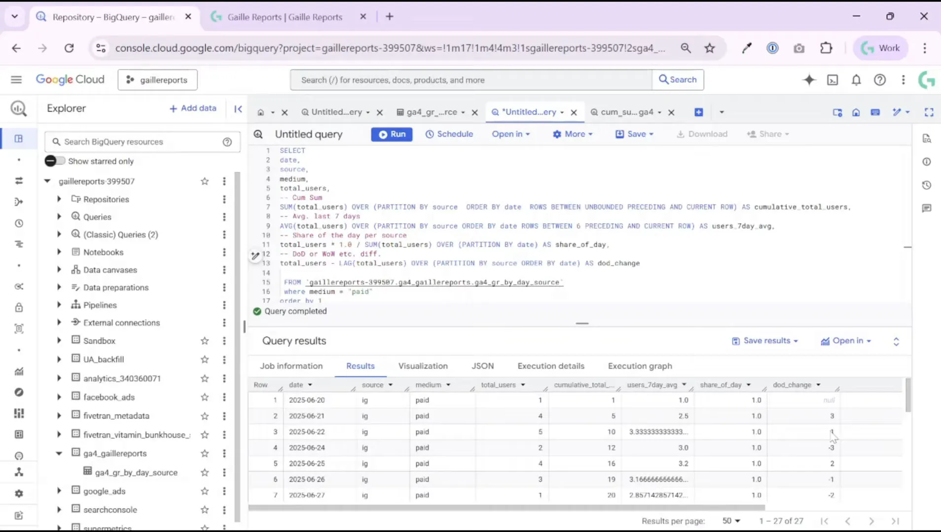
Step 4: Calculate day-over-day (or week-over-week) difference and percent change
Day-over-day (DoD) deltas and percent changes are fundamental in time series analysis. To calculate the difference between a day and its previous day you use the LAG() function. A common pattern is:
total_users - LAG(total_users) OVER (PARTITION BY source ORDER BY date) AS users_diffIf you want percent change, you divide the diff by the previous day’s value (watch out for zeroes) like this:
((total_users - LAG(total_users) OVER (...)) / LAG(total_users) OVER (...)) * 100 AS users_pct_changeExample from the dataset:
- 20 June — no previous day, so DoD is NULL.
- 21 June — 4 users vs previous 1 → difference = 3 (we gained 3 users).
- 22 June — 5 users vs previous 4 → difference = 1 (gained 1 user).
- 23 June — 2 users vs previous 5 → difference = -3 (lost 3 users).
These simple numbers help you spot where attention is needed: a sustained negative DoD or multiple negative weeks could indicate tracking issues, campaign exhaustion, or UX problems causing drop-offs.
Step 5: Extend these patterns to revenue, CLV, and other metrics
The window function patterns I showed aren’t limited to users. Replace total_users with revenue, purchases, or average_purchase_per_customer and the same logic applies. For example, compute a customer-level lifetime value by partitioning by customer_id and using cumulative SUM or moving averages to smooth revenue per user over time.
Examples to try:
- Customer lifetime revenue: SUM(revenue) OVER (PARTITION BY customer_id ORDER BY date ROWS BETWEEN UNBOUNDED PRECEDING AND CURRENT ROW)
- 7-day average revenue per user by source: AVG(revenue) OVER (PARTITION BY source ORDER BY date ROWS BETWEEN 6 PRECEDING AND CURRENT ROW)
- Share of revenue by campaign each day: revenue / SUM(revenue) OVER (PARTITION BY date)
These metrics feed directly into dashboards in Looker Studio, where you can create time series charts for moving averages, stacked area charts for daily shares, and KPI tiles showing DoD or WoW changes. I often compute these in BigQuery and surface the pre-aggregated results in Looker Studio for fast reporting.
Practical tips and pitfalls
- Always partition your window functions by the correct dimension (source, customer_id, campaign). Wrong partitioning mixes groups and produces misleading metrics.
- Watch out for division by zero when computing percent change — handle zeros with SAFE_DIVIDE or CASE statements.
- Use scheduled queries to maintain a compact daily table rather than running heavy event-level queries every time you need a report.
- Consider using CAST or multiplying by 1.0 to force floating-point division when computing shares or percentages.
- Keep your date ordering consistent — if you have multiple time zones or datetime columns, normalize to DATE to avoid ordering mistakes.
Wrap-up and next steps
These window function patterns unlock a lot of practical analytics: moving averages to smooth noise, daily share to monitor channel mix, and lag-based differences to spot short-term changes. Once you generate these values in BigQuery, push them into Looker Studio for visual reports or connect them to downstream tools.
If you want to reproduce the examples I used in this article, here are the core SQL patterns again (in words):
- 7-day moving average per source — AVG(…) OVER (PARTITION BY source ORDER BY date ROWS BETWEEN 6 PRECEDING AND CURRENT ROW)
- Daily share per source — total_users / SUM(total_users) OVER (PARTITION BY date)
- Day-over-day difference — total_users – LAG(total_users) OVER (PARTITION BY source ORDER BY date)
I hope you had as much fun following these tricks as I had when I discovered them. These calculations are small but incredibly useful when you need to translate event-level noise into reliable business metrics.
Recommended reading on Gaille Reports
If you liked this article, check out these related posts and guides on my site:
- How to Automate GA4 Reports in BigQuery with Scheduled Queries
- BigQuery GA4 Users Sessions Tutorial: How to Identify Your Top Traffic Sources
- How to Use SQL with GA4 in BigQuery: 10 Real Examples for Marketers
- How to Use Looker Studio: Beginner Guide (2025)
If you want help translating these patterns to your data model (different column names, custom customer_id, or campaign mapping), drop a note on the blog or reach out via the Gaille Reports contact channels. I often publish templates and Looker Studio examples that use the exact BigQuery queries I show here.
Pro tip: If you need to bring data into BigQuery from multiple platforms, consider using an API connector.
Windsor.ai lets you connect ad platforms like Facebook, Google Ads, LinkedIn and more directly to BigQuery.
Use promo code gaillereports to get 10% off any Windsor.ai plan.