How to Calculate Running Totals in BigQuery (GA4)

I love turning raw GA4 data in BigQuery into actionable metrics, and one of the most useful techniques I rely on is a cumulative sum (also called a running total). In this article I’ll walk you step-by-step through a practical example using a small GA4-derived table: how to calculate cumulative users (or revenue), how the SQL works, and how you can adapt the same pattern to compute customer lifetime value (CLV) or first-N-days metrics (for example, the first 90 days after sign-up).

If you prefer the video walkthrough, watch the tutorial here:

Step 1: Inspect the dataset and define the use case

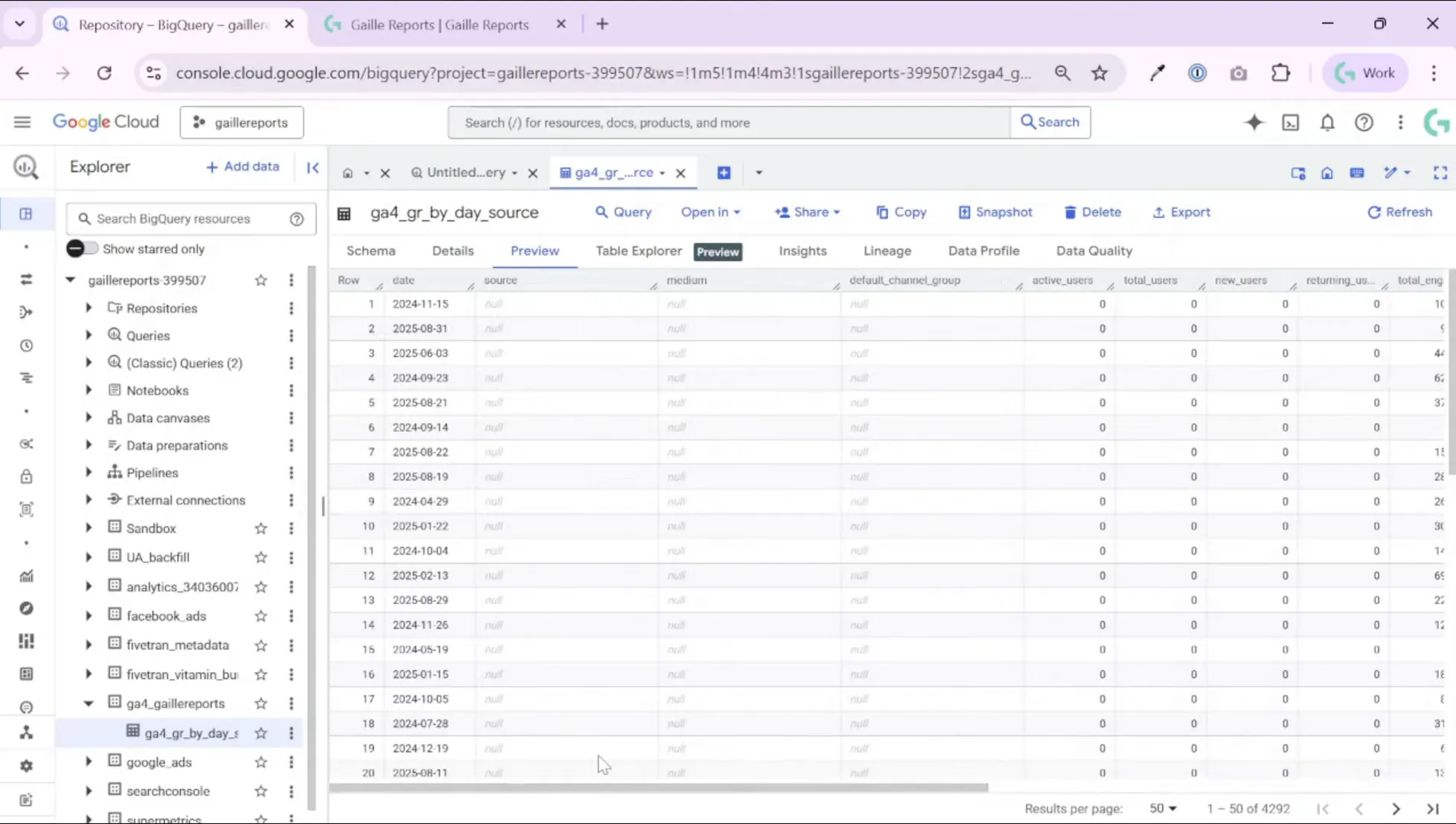
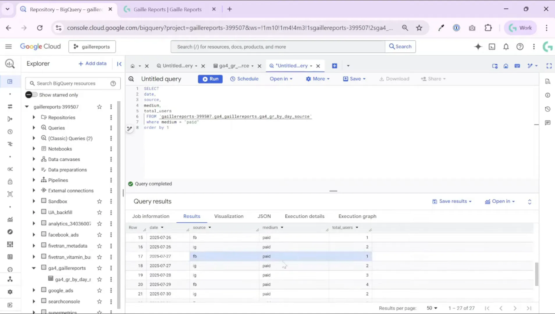
Start by understanding the table you’ll query. In my example, I rebuilt a smaller GA4 table in BigQuery using a scheduled query so it’s easier to demo. The table contains at least these columns:

date (event or session date)
source_medium (or source + medium combined)
total_users (or a metric like purchase_amount / revenue)

I filtered the dataset to one campaign type — medium = ‘paid’ — so we only look at paid traffic. The preview shows daily rows with date, source/medium, and users. That’s all we need to produce a cumulative sum by day and by source.

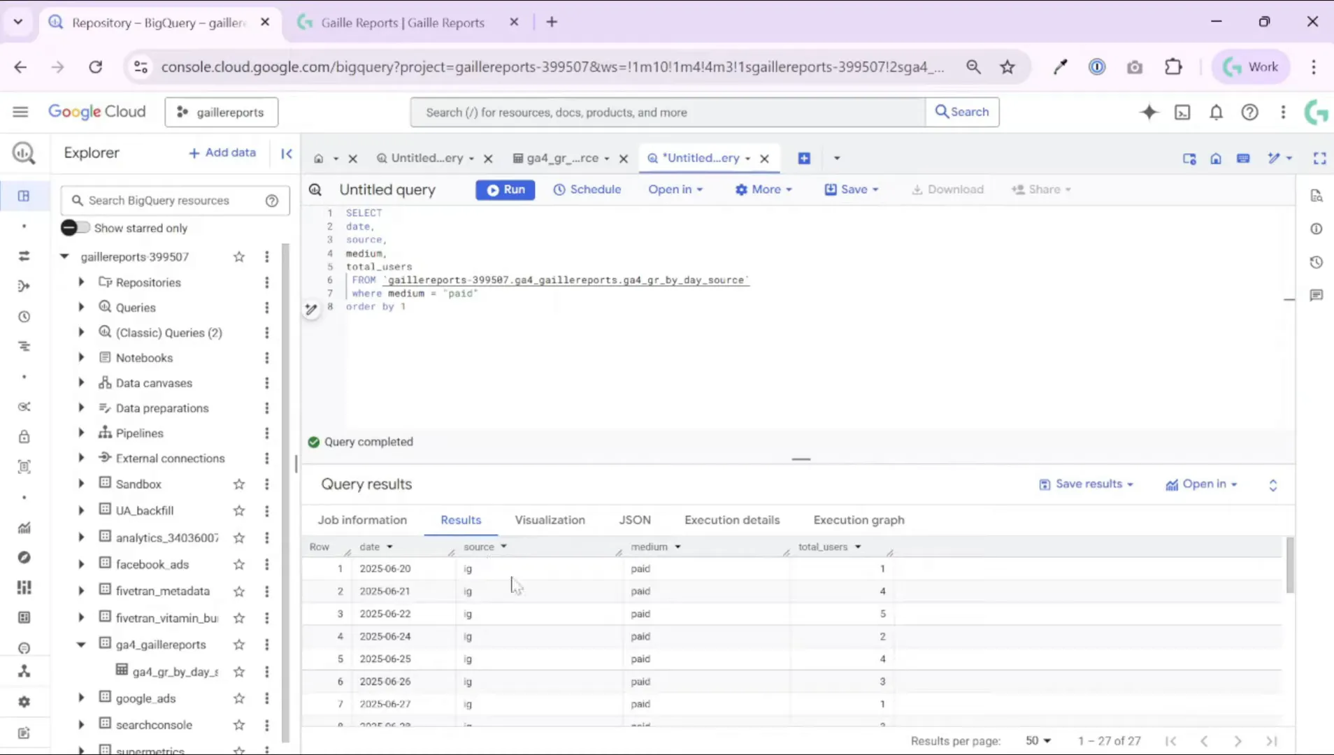
Preview of BigQuery table: date, users, source_medium

Step 2: Write the basic cumulative SQL query

The core idea is to use a window function with SUM(…) OVER(…) so BigQuery calculates a running total for each partition. Here is a compact example you can adapt (replace project.dataset.table with your table):

Example SQL (cumulative users by source and day)

SELECT
date,
source_medium,
total_users,
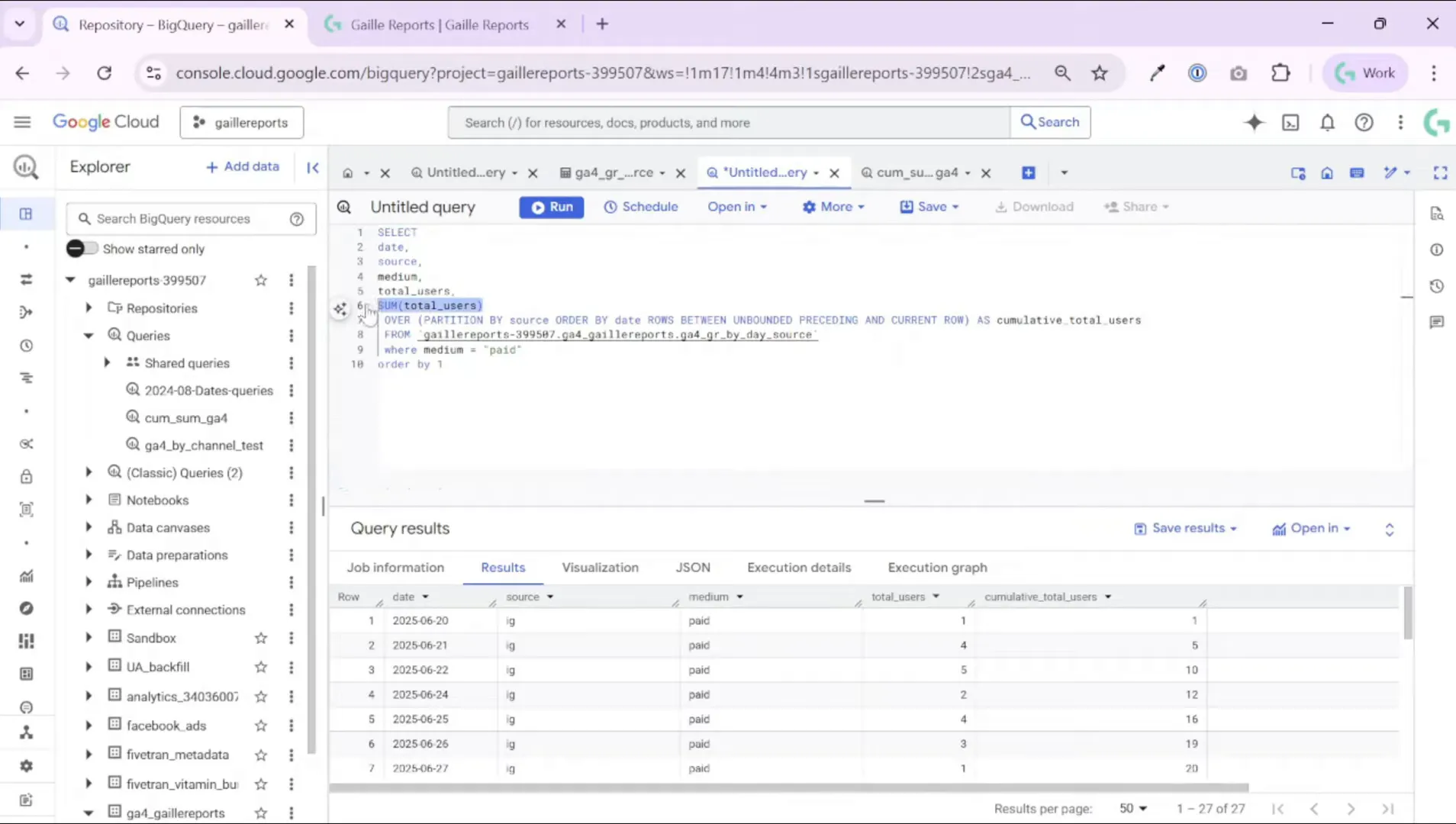
SUM(total_users) OVER (PARTITION BY source_medium ORDER BY date ROWS BETWEEN UNBOUNDED PRECEDING AND CURRENT ROW) AS cumulative_users
FROM `project.dataset.table`
WHERE medium = 'paid'
ORDER BY source_medium, date;

Key parts explained:

SUM(total_users): the metric you want to accumulate. If you track revenue, replace total_users with revenue or purchase_amount.
OVER (PARTITION BY source_medium …): partitioning ensures we compute separate running totals for Instagram and Facebook (or any other dimension). Without partitioning, you’d mix all sources together.
ORDER BY date: the running total accumulates in chronological order.
ROWS BETWEEN UNBOUNDED PRECEDING AND CURRENT ROW: the frame tells BigQuery to start at the first row and run up to the current row (the classic cumulative/running behavior).

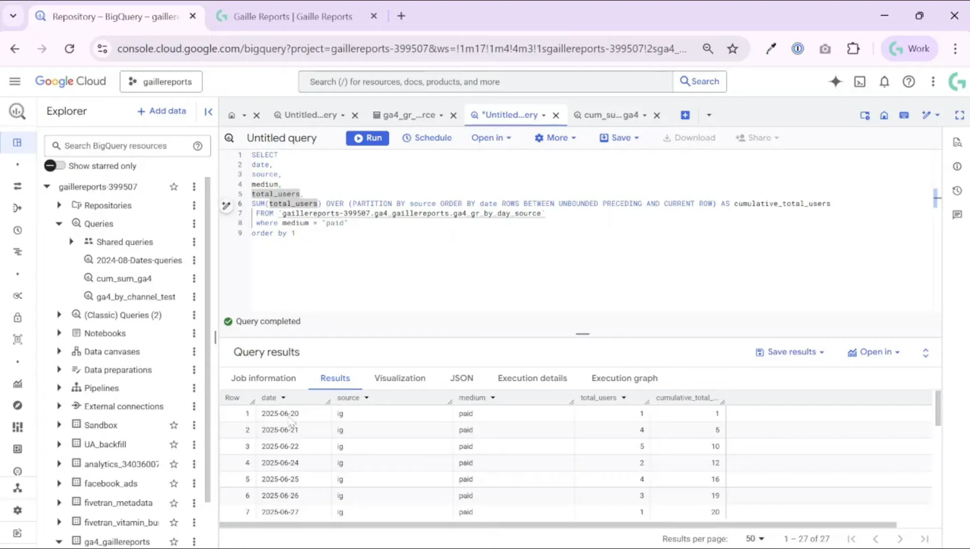
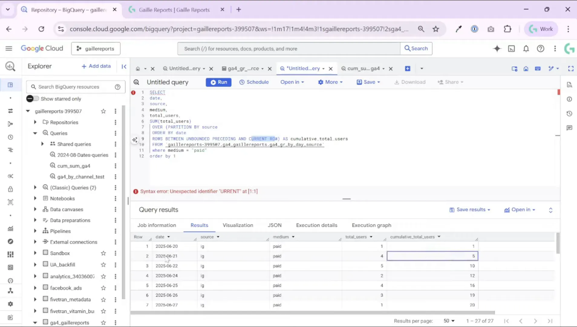
SQL editor preview showing cumulative SUM and OVER partitioning

Step 3: Run and read the results — how to interpret cumulative numbers

After you run the query, you’ll see that the cumulative column grows day by day for each partition. For example:

20 June: users = 1, cumulative_users = 1
21 June: users = 4, cumulative_users = 5 (1 + 4)
22 June: users = 5, cumulative_users = 10 (previous 5 + 5)

This pattern helps answer business questions such as “how many users did this campaign accumulate up to this date?” or “how much revenue did this channel generate within the first N days?”

Query results showing daily users and cumulative total per source

Step 4: Turn cumulative sums into CLV (cumulative revenue per user)

A very common and powerful adaptation is to calculate cumulative revenue per user to approximate customer lifetime value (CLV) over time. To do this, you typically partition by user_id instead of source, and order by event_date. That way the cumulative value represents how much each customer has spent up to each day.

Here’s a practical pattern:

SQL to compute cumulative revenue per user

WITH base AS (
SELECT user_id, event_date, revenue
FROM `project.dataset.events_table`
WHERE revenue IS NOT NULL
),
cum AS (
SELECT
user_id,
event_date,
revenue,
SUM(revenue) OVER (PARTITION BY user_id ORDER BY event_date ROWS BETWEEN UNBOUNDED PRECEDING AND CURRENT ROW) AS cumulative_revenue
FROM base
)
SELECT * FROM cum ORDER BY user_id, event_date;

That result gives you a timeline per user, showing how their cumulative spending grows. You can then aggregate across users to get cohort CLV (e.g., average cumulative revenue per user by cohort day).

Example partitioning by user_id to see per-user cumulative revenue (CLV)

Step 5: Limit to first N days after signup (e.g., 90-day CLV)

Often, you want cumulative metrics for a fixed window after the user’s first event (for example, the first 90 days after sign-up). You can compute the user’s first_date with a window MIN(), then filter rows where the date difference stays within your window.

SQL: cumulative revenue for first 90 days per user

WITH base AS (
SELECT
user_id,
event_date,
revenue,
MIN(event_date) OVER (PARTITION BY user_id) AS first_date
FROM `project.dataset.events_table`
),
filtered AS (
SELECT *,
SUM(revenue) OVER (PARTITION BY user_id ORDER BY event_date ROWS BETWEEN UNBOUNDED PRECEDING AND CURRENT ROW) AS cumulative_revenue
FROM base
WHERE DATE_DIFF(event_date, first_date, DAY) <= 90
)
SELECT * FROM filtered ORDER BY user_id, event_date;

This returns only the events where the user is within their first 90 days, and the cumulative_revenue reflects totals up to each date inside that window. You can then calculate per-user totals at day 90 or average them to produce cohort CLV.

Step 6: Practical tips & performance considerations

Window functions are powerful, but you should watch out for query cost and performance on very large tables. Here are practical tips I use:

Filter early: push WHERE clauses (e.g., medium = ‘paid’, date ranges) into a subquery to reduce row counts before window computations.
Limit columns: select only the columns you need (user_id, date, revenue) to reduce processed bytes.
Use scheduled queries to pre-aggregate or rebuild lightweight tables that contain daily metrics. I often rebuild a small table (one row per date + metric) and use that for dashboards — it saves repeated heavy processing.
Partition and cluster your BigQuery table by date and by the most-used dimensions (user_id, source_medium). This helps cost and performance when filtering and ordering.
When dealing with millions of users, consider computing per-user cumulative totals offline (scheduled job) and storing results in a summary table to serve dashboards quickly.

Example showing daily accumulation and the concept of unbounded preceding to current row

Step 7: Common variations you’ll want to try

Partition by campaign or creative_id to see campaign-level accumulations.
Compute cumulative counts of conversions, not only users or revenue.
Create cohort views: use the user’s acquisition date as a cohort and compute cumulative revenue per cohort day.
Combine window functions with ROW_NUMBER() or RANK() to pick the first N occurrences per user (for example, first purchase event).

Daily rows by source (Instagram, Facebook) to illustrate partitioning

Quick checklist before you run the query

Have you limited the date range?
Did you filter out irrelevant mediums/sources early?
Is the partition dimension chosen correctly (user_id vs source)?
Are you ordering by the correct date column?
Do you want to persist results to a table via a scheduled query?

Final thoughts (summary)

Window functions in BigQuery let you write concise SQL to compute running totals and cumulative metrics. In practice, I use this approach for:

Daily cumulative users or conversions per channel
Per-user cumulative revenue to estimate CLV
First-N-days cohort analysis (for example, 90-day revenue)

Remember to partition by the right dimension (source or user), order by date, and use the frame ROWS BETWEEN UNBOUNDED PRECEDING AND CURRENT ROW for a classic running total. For large datasets, pre-aggregate with scheduled queries and use table partitioning/clustering to control cost and speed.

If you want to follow up with the practical steps I used to prepare the GA4 table in BigQuery (scheduled queries and rebuilding a compact table), check those resources and examples on the blog.