How to use the VLOOKUP function in Google Sheets?

When working with interrelated data, one of the foremost common challenges is finding data over different sheets. You frequently perform such tasks in everyday life, for example when checking a flight plan board for your flight number to induce the departure time and status. Google Sheets VLOOKUP works in a comparative way – looks up and recovers coordinating information from another table on the same sheet or from a distinctive sheet.

Check out the video tutorial here:

Let’s see how it works in practice

You have two databases – the one with people’s orders and the other one with order status.

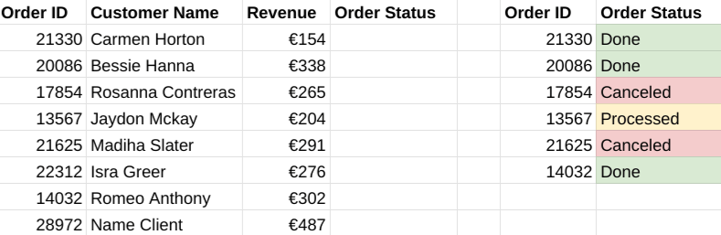
To make VLOOKUP function, it is really necessary to have a сommon column in both of the tables so that we could match them. Each row (each order) needs to have a personal and unique number or date, that would distinguish one row from another. 

Our task is to add the order status from the second database to the first one. How can we do it?

Having selected the cell with the order status that needs to be filled, I write a formula:

=VLOOKUP(A4,F3:G9,2,0)

Basically, this formula means that we need to find the data corresponding to the cell A4 in the data range F3:G9, taking into consideration only the second column of the F3:G9 data range.

To be able to apply this formula to the whole data range I simply transform this formula by adding dollar signs, so now the formula looks like this:

=VLOOKUP($A4,$F$3:$G$9,2,0)

Fixing the errors

But, we don’t have all the order IDs matching in both of the databases. That is why when there is an order ID in the first table and there is no correspondence in another one, after applying the VLOOKUP formula we will have errors. It is really bad, and it is better to change the missing data to “null” or something else. 

We can fix it! To do this, we need to transform our formula to the following one:

=IFERROR(VLOOKUP(A4,F3:G9,2,0), “Not found”)

This, in fact, means that when there is going to be any missing data, the cell will contain “Not found” text. 

You also can read an article about the usage of ARRAYFORMULA with the same table.

If you want to know more about Looker Studio and start your life changing freelancing data visualization career, you are more than welcome to my Gaille Reports course. Read more about it here. 

You can also read more articles of mine in Medium.

Hope this tutorial was interesting and useful for you! Don’t hesitate to write your impressions in the comments section.