How to use ARRAYFORMULA in Google Sheets?

Google Sheets is a great tool that I use everyday in my work and as we all know it has plenty of formulas that easen our routine tasks and one of the formulas that I find really interesting and useful is ARRAYFORMULA. In this article I would love to tell you about ARRAYFORMULA and the regular ones. Let’s start!

If you like video format, here is the tutorial:

Differences

Basically, regular formulas are applied just to one cell. To spread it to other cells, we can just duplicate this formula and it is fine if you have a stable data range. However, in my case, I usually connect my Google Sheets to Looker Studio and I always need only fresh data. For this reason I use APIs that pull up the most relevant data to Google Sheets and, consequently, my data range is only expanding. Here is when ARRAYFORMULA in Google Sheets comes in!

Let’s take a look at the example

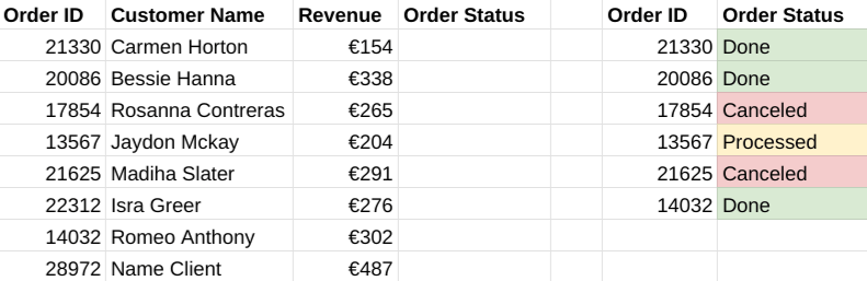
Here we have two tables and both of them contain Order ID. Our task is to match Order ID and Order Status from the first table using the second table. We could use VLOOKUP formula if we had a stable data range, it would look like this: 

=VLOOKUP($A4,$F$3:$G$9,2,0)

You can read more about the VLOOKUP formula in this article (link). 

In our case, when the data is constantly updating, we need to use the ARRAYFORMULA that will look this way:

=ARRAYFORMULA( VLOOKUP($A4:A,$F$3:$G$9,2,0)

I’ve made the change in the formula bold and underlined – that is how we applied the formula to the whole column of the data range. But it also applies to completely empty rows that don’t contain any data and we get the errors in the table so, as a consequence, I will not be able to add this table to Looker Studio because I will see only broken charts. Let’s fix it. 

Avoiding errors

Firstly, we have a way to apply the formula only to the rows that contain some information. We just need to transform our formula this way:

=ARRAYFORMULA( IF A4:A = “ “, “ “ , VLOOKUP($A4:A,$F$3:$G$9,2,0)

We still have errors in the cells that didn’t find any matching data from the second table, but at least we don’t have the errors throughout the whole tab. To avoid all the errors, we just add IFERROR to the formula. So the final formula in our case looks like this:

=ARRAYFORMULA( IF A4:A = “ “, “ “ , iferror(VLOOKUP(A4:A,$F$3:$G$9,2,0)))

If you want to know more about Looker Studio and start your life changing freelancing data visualization career, you are more than welcome to my Gaille Reports course. Read more about it here.

You can also read more articles of mine in Medium.

I hope this article was useful for you. Do not hesitate to write your impressions in the comments section!