How to convert currency in Google Sheets by a specific date using Googlefinance formula?

Have you ever faced an issue while working in Google Sheets when you need to convert cost or revenue from one currency to another? It is much easier than you may think because Google Sheets has a special function for it! Enjoy reading, I will explain!
Or if you prefer video format, check out a youtube tutorial:
Pre-setup
Let’s talk more about the formulas. Basically, there are two options and they are quite similar. The formula we will use to work with currencies is =GOOGLEFINANCE. It is a really powerful formula that allows you to do various things but we will use it in the simplest way – currency conversion.
Googlefinance. Formula 1

That is how the first formula looks like. Here we wrote which currency we want to convert into which one. We will convert USD to EUR. The formula automatically converts currencies and returns us the result of the current exchange rate, in this case it is 0.8987
Googlefinance. Formula 2

Using this formula we do not write the codes of the currencies but we select the cells containing these codes instead. In the image we can see that in the formula I have selected first cell “From” then cell “To” and we got the result in the column “Rate”.
Example
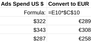
When we have a certain metric, for example Ads Spend in USD, and we need to show this metric in other currencies, like EUR or CAD, using calculated rate, we just multiply it to the value of the metric. Check out the formula and how the Ads Spend is being converted in EUR.

Case
Currency rates are being updated every 20 minutes, so every time you will see different numbers in the Sheets.
Personally, I frequently work with the cases when I have dates and, for example, cost in USD that I need to transform to EUR considering the currency rate of that date.
In this case the formula gets slightly more complicated. Let’s have a look at it.
=GOOGLEFINANCE(“Currency:USDEUR”, “price”, [Date Start], [Date End])
As you can see, here we add some attributes, like price, Date Start and Date End. If you go to Google Sheets Support page, you can find a list of different attributes you can use.
There are three different ways you can write this formula.

The differences between them:
- The first example contains the codes of the currencies, price attribute, numeric date and Today as a Date End.
- The second formula contains cell links instead of codes – the rest is basically the same.
- The third formula contains the links to the cells instead of currency codes or Date Start/Date Finish.
As a Date Start/ Date Finish in the third example I have used minimum and maximum dates of our date range. To do it, I created two columns, named them Min Date and Max Date, and used formulas:
=min(A31:A35)
=max(A31:A35)
Formula for the To Date Column looks like this:
=TO_DATE(int(B21))
Applying formulas
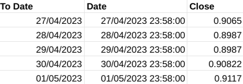
After applying this formula to the date range, that’s what we will get:

We don’t need time in the Date column. To fix it we need to write a formula that looks like this:
=TO_DATE(int(B21))
Finally, let’s take a look at our sample.

To find the exchange rate, we use the formula VLOOKUP, that in our case will look like this:
=VLOOKUP(A31,A21:C26,3,0)
This formula can be like this: A31 – date that we are looking for in our date range A21:C26, and use the exchange rate from column 3. To avoid any errors, I add IFERROR to the formula, so the final formula looks like this:
=IFERROR( VLOOKUP(A31,A21:C26,3,0),1)
And to get the cost in euro I just multiply the cost in USD to the exchange rate that we got.
Hope you liked this tutorial! Do not hesitate to leave the impressions in the comments section!
