Google Sheets Logic Functions: Full Overview (IF, IFS, AND, OR Explained)

Google Sheets logic functions are powerful tools that allow you to make your spreadsheets smarter and more dynamic. Whether you’re analyzing data, automating tasks, or solving complex problems, functions like IF, IFS, AND, and OR provide the flexibility to implement conditional logic with ease. 

But before we start, check out the video tutorial for a better understanding!

I’ve created such a table for us to practice with marketing data. 

IF Function

Let’s start with the most basic but not the least important IF function.

=IF(logical_expression, value_if_true, value_if_false)

Logical expressions

Using this formula you can validate just one logical expression. As a logical expression you may use different types of data:

1. Word containing logical expressions: C3=”New”. 

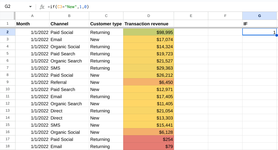
If the statement is true the value will be 1, if the statement is false, the value returned will be 0. NOTE: the result values may be either numeric, textual or a formula. 

2. Cell comparison: C3=H2 (if we write a certain word in the cell H2, for example “New”, so it basically turns into a word containing logical expression we’ve seen above)
3. More (>) or less (<) signs. It works with numeric data in the cell. For instance, =IF(D2>10000, 1, 0)

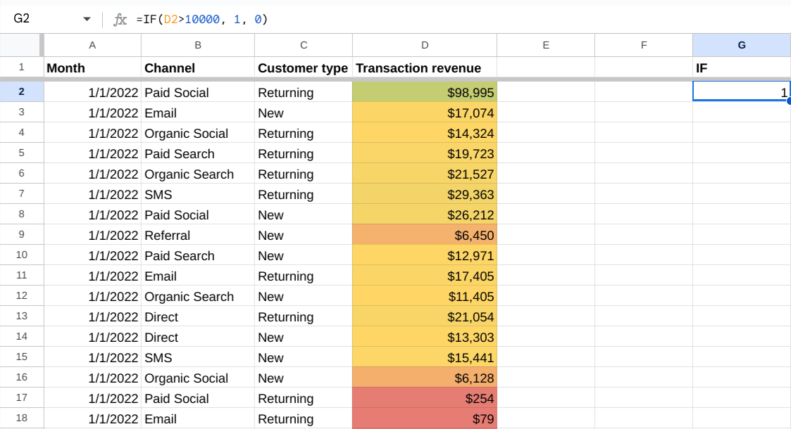
If the revenue from the cell D2 is bigger than 10000, the returned value will be 1, if the statement is false, the value will be 0.

Nesting for several conditions

If we have several conditions we’d like to check, we can try nesting the formula (writing one formula inside the other).

Let’s say, we need to check whether the Channel C2=”Returning” and whether the Revenue D2>10000. If both of the conditions are met, the result will be “Good”, if not – “No” Hence, we make a complex formula:

=IF(C2=”Returning”,IF(D2>10000, “Good, “No”), “new”)

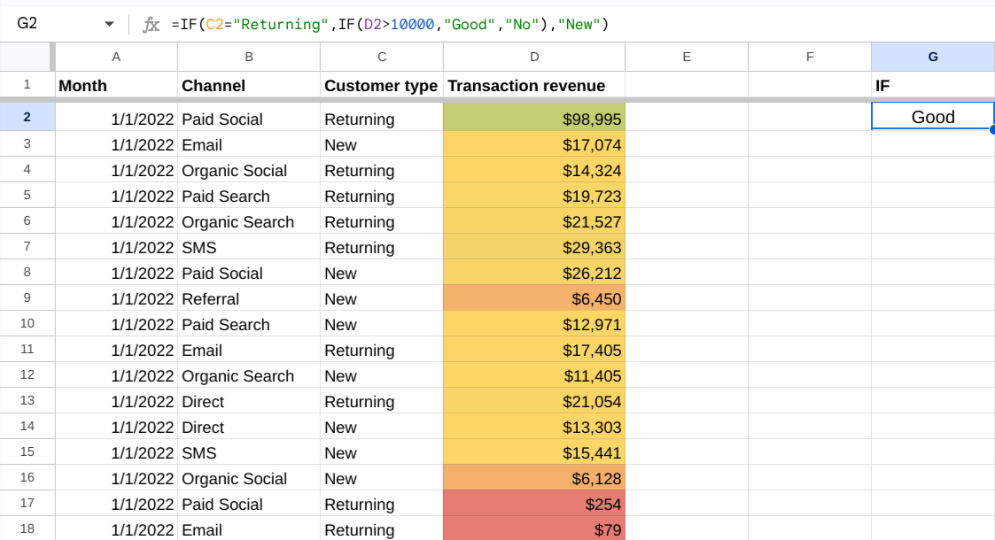
This is how if all the conditions are met, the result will be “Good”, if the second is not met – “No”, if none of the conditions – “new”.

AND Function

The AND formula in Google Sheets is used to evaluate multiple conditions and return TRUE only if all the conditions are met. It’s a logical function that helps you test whether multiple criteria are simultaneously true. If even one condition is false, the function returns FALSE.

We can literally check unlimited conditions at the same time and with the help of the IF Function it’s also a bit easier to do.

=IF(AND(C2=”New”, D2>10000), 10,0)

That’s pretty much the formula from the nesting example – the only things different are the values if true (10) and if false (0), but that doesn’t change anything. 

OR Function

The OR formula in Google Sheets is used to test multiple conditions and returns TRUE if at least one of the conditions is met; otherwise, it returns FALSE. It’s especially useful when you need to evaluate several criteria and take action if any of them are satisfied.

=IF(OR(C2=”New”, D2>10000), 10,0)

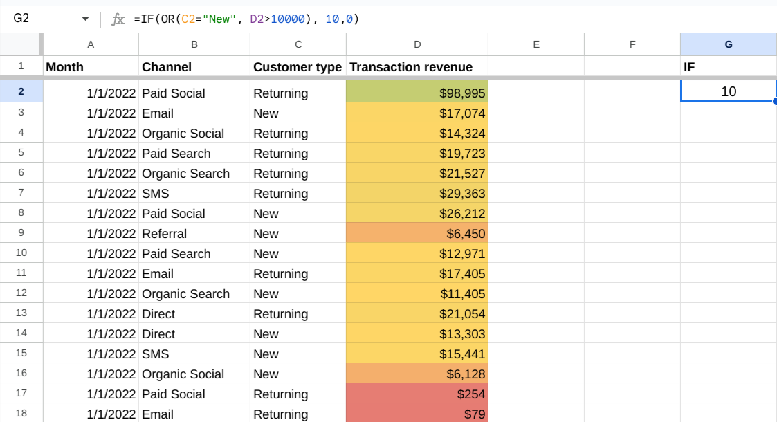
If we use the same formula, just change AND to OR, it will mean that if only one of the conditions is met, the result will already be positive.

IFS Function 

The IFS formula in Google Sheets is used to evaluate multiple conditions and return a value corresponding to the first condition that is true. It simplifies the process of writing nested IF statements, making your formulas easier to read and manage when dealing with multiple criteria.

Basically, it resembles the combination of the IF and AND functions. 

It works by this algorithm: if condition 1 is true, we use value 1; if it is false, check condition 2. 

For instance:

=IFS(D2>=50000, “The Best”, D2>=20000, “Great”, D2>=10000, “Good”)

Verbalizing this formula, if the Revenue in the cell D2 is rather than 50000, return “The Best”, if it’s rather than 20000, then return “Great”, and if it’s rather than 10000, then return “Good”.

If we structured the formula differently, like checking D2 >= 10000 first, it would result in incorrect outputs for higher values (e.g., D2 = 50000 would return “Good” instead of “The Best”). By checking the highest threshold first, we ensure that higher priority conditions are handled before lower ones

Working with Arrays

IF function perfectly combines with the ARRAY formula, so if we substitute the cells with the data ranges, it will be all good:

=ARRAYFORMULA(IF(C2:C10=”Returning”,IF(D2:D10>10000, “Good, “No”), “new”))

However, if we try to do the same trick with the AND formula, it will not work like this. 

The AND function is not array-compatible. It evaluates all the conditions together and returns a single TRUE or FALSE result for the entire range, not for each row.

When you try to use AND in an ARRAYFORMULA, it treats the entire range (e.g., D2:D10>10000) as a single logical value, which breaks the row-by-row evaluation needed for arrays.

The same thing applies to OR and IFS, they are not going to work with data ranges. 

Conclusion

The AND, OR, IF and IFS functions are one of the vital functions to know for the marketers who work with data in Google Sheets. When combined with the other logical functions it reveals a lot of opportunities for data analysis. 

Did you like this article? Follow my YouTube channel to be among the first ones to watch the new videos!

By the way, if you haven’t subscribed to my newsletter yet, do it right now and get a Looker Studio template for free!