Google Sheets: Learn the IFS Function with Easy Examples

Have you ever felt the need to use several conditions when working with the IF function? Most likely you surely have. In this article I am going to tell you everything you need to know about the IFS function, which is a bit more complex and advanced version of the basic IF formula.

Difference between IF and IFS

First of all, these two functions are built slightly differently and serve for different purposes.

=IF(logical_expression, value_if_true, value_if_false)

Using this formula you can validate just one logical expression. Whereas using IFS you can validate various expressions.

=IFS(condition1, value1, [condition2, …], [value2, …])

Basically, it works by this algorithm: if condition 1 is true, we use value 1; if it is false, check condition 2.

Using the formula in practice

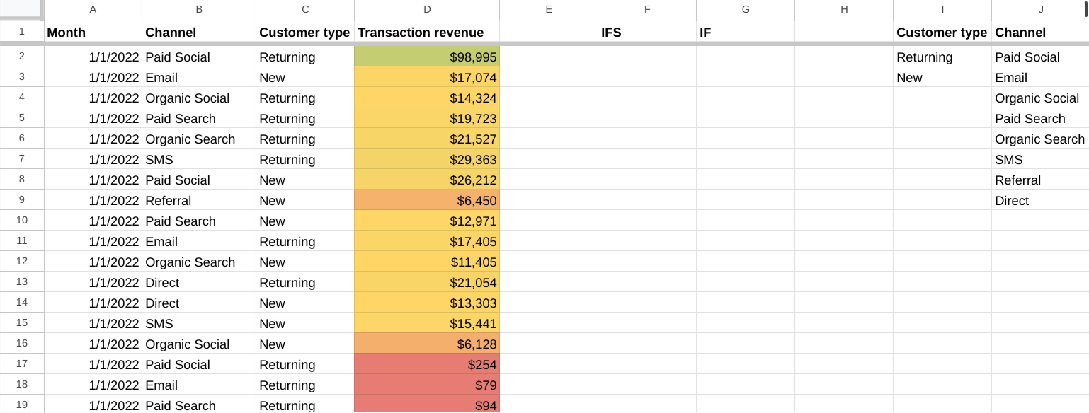
We have such a table showing date, channel, customer type and transaction revenue. And there is also an additional table that will help us compose a formula and will serve as conditions.

So the first example in this case:

=IFS(B2=J2, “Paid”)

Verbalising this formula, if a field B2 is the same as field J2, the result will be “Paid”. We can lock the cell by changing J2 to $J$2, so that when applying this formula to the column, it will not change. We need it, because it’s a condition. However, if we want to apply this formula to other rows from the table, we need to extend the formula, otherwise we will have errors.

Extending formula

Using IFERROR

Let’s extend this formula and get rid of the errors by using the IFERROR formula.

=IFERROR(IFS(B2=J2, “Paid”), “Other”)

So if the content of the cell is not equal to J2 (Paid), the result will be “Other”.

Adding more conditions

As we have a list of conditions we can use, let’s extend the IFS part of the formula.

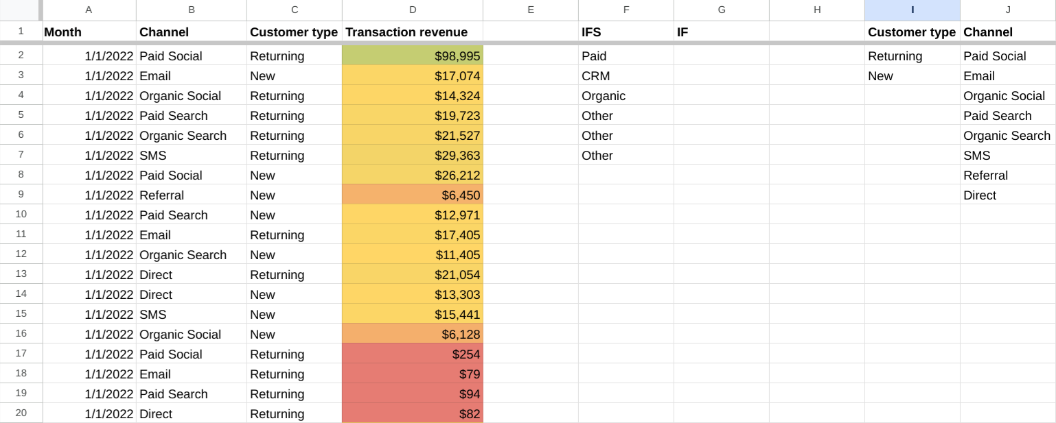
=IFERROR(IFS(B2=$J$2,”Paid”,B2=$J$3,”CRM”,B2=$J$4, “Organic”),”Other”)

If B2 is the same as J2, the result will be “Paid”. If not, let’s compare it with J3. If they match, the result will be “CRM”. But if none of the existing conditions match the field, to avoid errors we will see “Other” as a result.

Using IF function

In addition, you also can try using the IF function in this case.

=if(B2=J2,if(C2=I2, 1,0),0)

In simple words, if Channel from column B matches the Channel from column J, let’s check if Customer types are also matched. If yes, the result will be 1, if no, the result will be 2. If Channel from column B doesn’t match the Channel from column J, the result will be 0.

Tip: Data Ranges (Array Formula)

IF function perfectly combines with the ARRAY formula, so if we substitute the cells with the data ranges, it will be all good:

=ARRAYFORMULA(IF(C2:C10=”Returning”,IF(D2:D10>10000, “Good, “No”), “new”))

However, if we try to do the same trick with the IFS formula, it will not work like this.

The IFS function is not array-compatible. It evaluates all the conditions together and returns a single TRUE or FALSE result for the entire range, not for each row.

When you try to use IFS in an ARRAYFORMULA, it treats the entire range (e.g., D2:D10>10000) as a single logical value, which breaks the row-by-row evaluation needed for arrays.

Conclusion

IFS function is one of the vital functions to know for the marketers who work with data in Google Sheets. When combined with the other logical functions it reveals a lot of opportunities for data analysis.

Did you like this article? Follow my YouTube channel to be among the first ones to watch the new videos!

By the way, if you haven’t subscribed to my newsletter yet, do it right now and get a Looker Studio template for free!